Theoretical Background

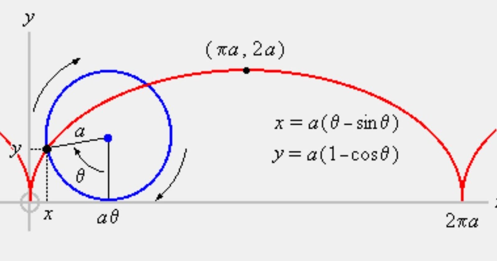
The cycloid motion is a very curious motion. It literally translates to the motion of a particle on the rim of a tyre of a cycle (hence, the name cycloid, duh!) Now, one may think, it makes no sense! It's just a circular motion. Technically, that person would be right had the cycle stayed at one place. Upon, a little more closer observation, we realise that the particle is having a translational(a fancy term for saying, 1D motion) component for its motion along with a rotational component.

Here, we will attempt to get a mathematical understanding of the motion and then model it using Python.

Let a constant magnetic field B be oriented along the x-axis and a constant electric field E along the z-axis.

Quick fact: An arrangement of this type is used in a planar magnetron.

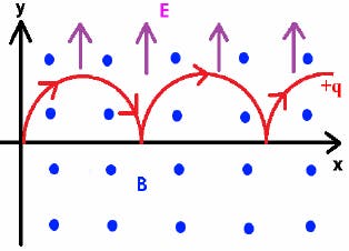
A positive charge of mass m and charge q is held at the origin of coordinates at time t = 0.

Initially, the particle is at rest, so no magnetic force acts on the particle. But, an electric force acts. and accelerates the charge in the positive z-direction by a force given by:

\[ \vec{F_E} = q \vec{E} \]

As the velocity v increases, the particle also experiences an additional force due to the magnetic field, which pulls the charge to the right. This force is given as \[ \vec{F_B} = q(\vec{v} \times \vec{B}) \]

An important thing to note here is that the particle's motion is constrained in the y-z plane as the forces acting on the particle are in the y-z plane.

We can write the velocity vector \(\vec{v}\) of the particle as \[ \vec{v} = \dot{y} \hat{e}_x + \dot{z} \hat{e}_y \]

Further, we have assumed that \(\vec{B} = B\hat{e}_x\) and \(\vec{E} = E\hat{e}_z \). Hence,

$$ \vec{F}_B = q\begin{vmatrix} \hat{e}_x & \hat{e}_y & \hat{e}_z\\ 0 & \dot{y} & \dot{z} \\ B & 0 & 0 \end{vmatrix} = q(B\dot{z}\hat{e}_y - B\dot{y} \hat{e}_y) $$

Applying Newton's second law, total force is $$ \vec{F} = \vec{F}_E + \vec{F}_B = qE\hat{e}_z + q(B\dot{z}\hat{e}_y - B\dot{y} \hat{e}_y) = m\vec{a} = m(\ddot{y} \hat{e}_y + \ddot{z}\hat{e}_z) $$

After, a little shuffling and equating terms, we get \[ \ddot{y} = \frac{qB}{m} \dot{z} = \omega \dot{z} \]

\[ \ddot{z} = \frac{q}{m}(E - B\dot{y}) = \omega \Big(\frac{E}{B} - \dot{y}\Big) \]

Here, \( \omega = \frac{qB}{m} \) is the same cyclotron frequency with which the particle revolve in the absence of an electric field.

So, we have a set of coupled differential equations. We can solve these and get our solution for the coordinates of the particle as a function of time numerically using the Scipy module (specifically, the odeint package).

Coding:

Working environment

I will be using Jupyter notebooks for my analysis because I need the ipywidgets module of Jupyter for tinkering with various parameters and initial conditions of the system which is more easily done using Ipywidgets.

Step 1: Import Packages

import numpy as np
import matplotlib.pyplot as plt
plt.style.use(['science', 'notebook', 'grid', 'dark_background'])
from scipy.integrate import odeint
import ipywidgets as widget
plt.rcParams['figure.figsize'] = (16, 5)

The most important package here is odeint which we will need for solving differential equations. Ipywidgets will provide an interface for tinkering with the hyper parameters of our solution.

Step 2: Design the ipywidgets wrapper

The wrapper will be used to solve the differential equations and plot them.

@widget.interact(Q = widget.FloatSlider(value = 5, min = 0, max = 20, step = 0.1,
                                       description = 'Charge Q'), 
                B = (0, 10, 0.1), E = (0, 10, 0.1), 
                 m = (0, 10, 0.1), 
                 nature = widget.ToggleButtons(options = [1, 0, -1], value = 1, 
                                              description = 'Charge'),
                 initial_y = widget.FloatSlider(value = 0, min = 0, max = 10, step = 0.1, 
                                                description = r'$y(t = 0)$'),
                initial_vy =widget.FloatSlider(value = 0, min = 0, max = 10, step = 0.01,
                                       description = r'$\dot{y}( t = 0)$'), 
                initial_z = widget.FloatSlider(value = 0, min = 0, max = 10, step = 0.01,
                                       description = r'$z(t = 0)$'), 
                initial_vz = widget.FloatSlider(value = 0, min = 0, max = 10, step = 0.01,
                                       description = r'$\dot{z}(t = 0)$'), 
                final_time= widget.FloatSlider(value = 10, min = 10, max = 50, step = 0.1,
                                       description = r'Time $t$'))

Two main elements here are:

• FloatSlider which gives a sliding knob for adjusting values
• ToggleButtons for changing values by clicking buttons

Step 3: Designing a function for the differential equations

First we imagine a vector \(\vec{S} \) containing everything that we want to solve for and pass the time derivative of this \(\frac{d\vec{S}}{dt} \) in our function. $$ \vec{S} = \begin{bmatrix} \dot{y} \\ y\\ \dot{z} \\ z \end{bmatrix} $$

def dSdt(S, t): # The ODE Equation
        y_dot, y, z_dot, z = S

        return [w*z_dot, # y''
                y_dot,   # y'
                w*(E/B - y_dot), # z''
                z_dot]   # z'

Step 4: Specify time for which to solve the equations and the initial conditions

As our solution is numeric so we need numeric data points over which we will solve our equations and need initial conditions for the position and velocity of the particle to eliminate the constants of the equations of motion.

ics = [initial_vy, initial_y, initial_vz, initial_z] # Initial conditions
t = np.linspace(0, final_time, 500) # Time range

Step 5: Solve the equations

This is easily done using the odeint pack

sols = odeint(func = dSdt, y0 = ics, t = t) # Solutions
y_vals, z_vals = sols.T[1], sols.T[3]

Step 6: Plot the solutions

We will perform this part using the famous Matplotlib library. The arrays are simple and easy to plot using generic Matplotlib commands.

plt.ylim(0, 0.65)
plt.xlim(-0.1, final_time+0.2)
plt.xlabel(r'$y\rightarrow$', fontsize = 18)
plt.ylabel(r'$z\rightarrow$', fontsize = 18)
plt.plot(y_vals, z_vals, lw = 4)

Step 7: Wrap everything up in a function to generate the interactive solution code

@widget.interact(Q = widget.FloatSlider(value = 5, min = 0, max = 20, step = 0.1,
                                       description = 'Charge Q'), 
                B = (0, 10, 0.1), E = (0, 10, 0.1), 
                 m = (0, 10, 0.1), 
                 nature = widget.ToggleButtons(options = [1, 0, -1], value = 1, 
                                              description = 'Charge'),
                 initial_y = widget.FloatSlider(value = 0, min = 0, max = 10, step = 0.1, 
                                                description = r'$y(t = 0)$'),
                initial_vy =widget.FloatSlider(value = 0, min = 0, max = 10, step = 0.01,
                                       description = r'$\dot{y}( t = 0)$'), 
                initial_z = widget.FloatSlider(value = 0, min = 0, max = 10, step = 0.01,
                                       description = r'$z(t = 0)$'), 
                initial_vz = widget.FloatSlider(value = 0, min = 0, max = 10, step = 0.01,
                                       description = r'$\dot{z}(t = 0)$'), 
                final_time= widget.FloatSlider(value = 10, min = 10, max = 50, step = 0.1,
                                       description = r'Time $t$'))

def CycloidMotion(Q, B, E, m, initial_y = 0, initial_vy = 0, initial_z = 0, initial_vz = 0, 
                  final_time = 10, nature = 1):
    Q = nature*Q
    w = Q*B/m # Angular Frequency

    ics = [initial_vy, initial_y, initial_vz, initial_z] # Initial conditions

    def dSdt(S, t): # The ODE Equation
        y_dot, y, z_dot, z = S

        return [w*z_dot, # y''
                y_dot,   # y'
                w*(E/B - y_dot), # z''
                z_dot]   # z'

    t = np.linspace(0, final_time, 500) # Time range
    sols = odeint(func = dSdt, y0 = ics, t = t) # Solutions

    y_vals, z_vals = sols.T[1], sols.T[3]
    plt.ylim(0, 0.65)
    plt.xlim(-0.1, final_time+0.2)
    plt.xlabel(r'$y\rightarrow$', fontsize = 18)
    plt.ylabel(r'$z\rightarrow$', fontsize = 18)

    plt.plot(y_vals, z_vals, lw = 4)

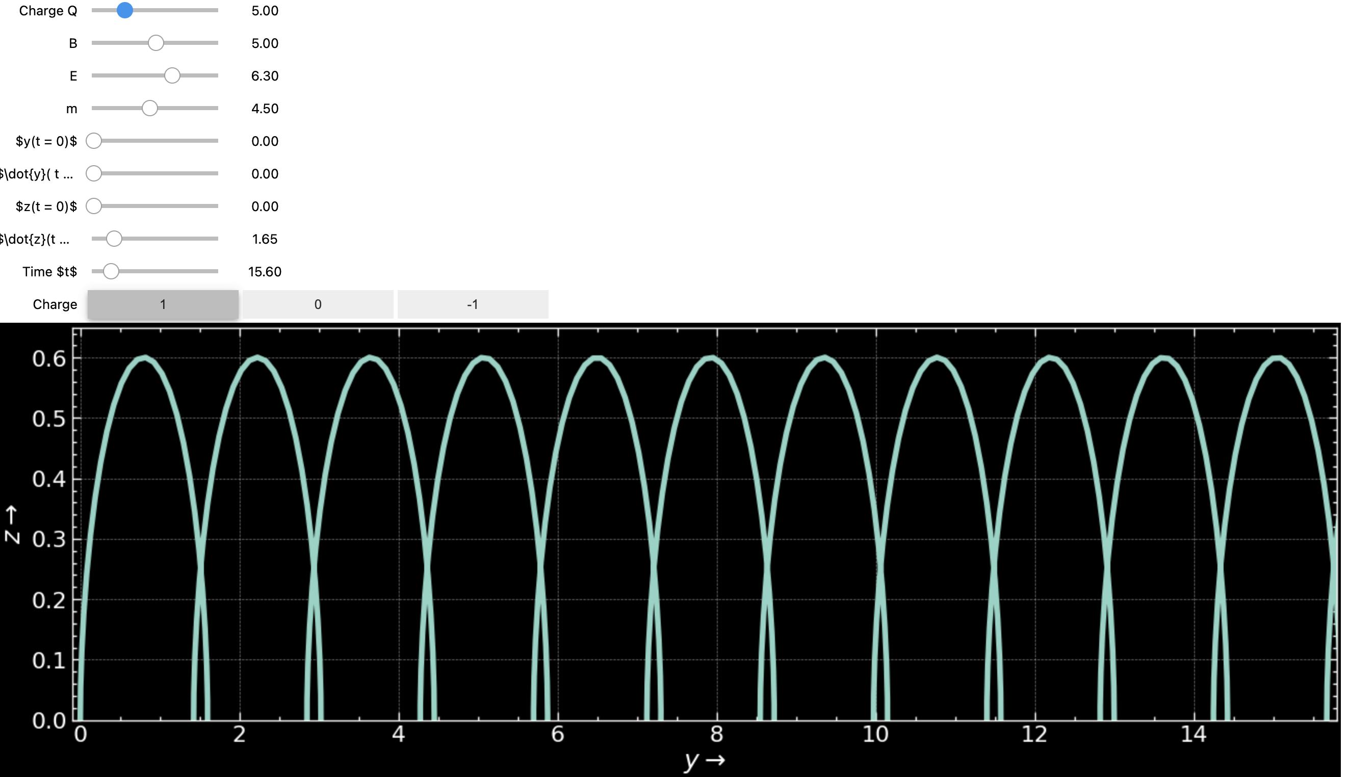
Solution Plot